
In the Drift: Issue 40, Spring 2021
In this issue
- FPOM
- Scientific Illustration for Freshwater Science
- SFS LRPC Request for Proposals
- Article Spotlight
- Children's Book
- Documentary Go Fund Me
- Book Review by Amy Rosemond
- Annual Meeting Recap
FPOM
SFS news and upcoming events collected from "the drift"
- Take the 2021 virtual meeting feedback survey
- Read the SFS President's Environment
- In Memoriam: David Ernest Ruiter (1948-2021)
- SFS Joint Meeting in Grand Rapids, MI (May 16-20, 2022)
- SFS Meeting in Brisbane, Australia (June 3-7, 2023)
2021 SFS Annual Meeting
By the numbers:
1140 -Total registrants (new record)
766 - Presentations (536 Oral, 230 Poster)
548 - Student registrants
229 - Registered fun runners
221 - Early career registrants
60 - Coffee breaks (855 Participants)
48 - Moderated discussions
32 - Countries represented
6 - Workshops
2 - Panel discussions
View meeting content until August 15
Scroll to the bottom of this issue for a photo recap.
Scientific illustration for freshwater science - a multi-part series
Part 2: Exposing the murky depths: Producing a scientific illustration
By Barrett Klein
Professor of animal behavior and entomology, University of Wisconsin – La Crosse https://www.uwlax.edu/profile/bklein/; http://www.pupating.org/
For some, science is daunting. For others, creating art can be daunting. Neither needs to be. If you revel in the rigors of conducting science, creating a scientific illustration is well within your grasp, if you give it some practice. For some thoughts as to why it might behoove you to create scientific illustrations, see part 1 of this series. For this installment, let’s consider how you can communicate your science by creating a scientific illustration. A comprehensive tutorial is not possible here, but if we begin with one type of illustration, any future illustration challenge will feel less intimidating. Follow along and try your hand at creating a scientific illustration that represents your research with clarity and visual appeal.
Visually depicting a message is like telling a story. Whether it takes the form of doodling on a board in front of colleagues while brainstorming ideas, or creating a figure for a poster, talk, or peer-reviewed publication, a story is often told best when following certain conventions, or meeting viewers’ sensory biases or expectations (Bang Wong wrote an excellent series of helpful guides in Nature Methods; see Wong 2011 as an example.). There are times to break from convention, but that discussion should not distract us here. I won’t speak of rules, but of guidelines that can help you deal with one common set of visualization challenges. Even if you claim not to be artistic, by practicing and following these guidelines you can render clearer, more accurate, and more effective visuals with practice.
ILLUSTRATION GUIDELINES 1) Observe your subject before you draw it. Know what structures or characteristics to look for and identify them before you pick up a pencil. Continue observing your subject as you create quick observational sketches. This can help ease you into the practice of more technical drawing. 2) Draw what you see. There is room for “artistic license” when interpreting your subject, but avoid compromising at the expense of accuracy. How much interpretation is necessary or acceptable depends on the subject and your audience. For example, if presented with fossilized dinosaur bones, do you draw them exactly as they appear to you, or assembled into an articulated skeleton, or as a fleshed-out, feather-bearing, live dinosaur on the run? It depends on your audience and what message you wish to impart. Here, we will be drawing what is in front of us, but as you’ll see, some flexibility exists (e.g., drawing a missing leg on an insect by creating a mirror image of an intact leg on the opposite side of the insect). 3) Scale your drawing to optimize clarity. Your drawing should fit comfortably within your drawing area – too small and you will not have enough room for detail, and an inability to reproduce your image at a reasonable size; too large and your subject will not fit in the designated area, and either you sacrifice portions of your subject, or force your subject to fit unnaturally into your drawing space. You can reduce the size of an image for reproduction/printing, but you cannot increase the size because it will quickly break down (unless you are creating a vector-based graphic, which is a digital drawing that can be scaled up indefinitely without loss of resolution). 4) If labeling structures, only label those that are visible. A viewer should be able to unambiguously identify each structure you label.
My starting point, to shake people free of their apprehensions, is to challenge them, without warning, to draw a portrait of the person beside them in the grand span of one minute. I keep everyone informed of their dwindling time remaining until it runs out, after which they exchange their drawings, amused and relieved that the challenge is over. There is little pressure here because, as I let them know afterwards, this is an unfair exercise, considering the time I gave them to depict a subject humans have evolutionarily been honed to instantly distinguish – the human face. Along with loosening up the artist-in-training, this exercise allows me to observe a person’s technique, and to highlight ways in which the technique could be improved. I introduce the guidelines, above, prior to the exercise, then return to these guidelines afterward, by presenting absurd and extreme, but instructional, examples of how I might epically fail with each.
CREATING A LINE DRAWING Scientific/technical illustrations are different than other drawings because they require you to make measurements and accurately depict proportions so that the end product accurately reflects reality. There are many ways to create a proportionally accurate illustration. One method is to draw a grid on your paper and place a grid in front of your subject (e.g., an optical grid in one ocular of a stereo/dissecting microscope will appear superimposed over the subject you are drawing) and match, square by square, the contents of what you see with what you draw. Another method is to use a camera lucida, which superimposes an image of your subject onto your drawing surface, allowing you to trace it. How you draw your subject can depend on whether or not the subject is large, alive or dead, asymmetrical, whether you wish to render it in color, etc. To simplify matters, we will create a black and white line drawing of a dead insect using a dissecting microscope, following a method that is different than those mentioned above. If you don’t have access to a dissecting microscope, the same principles and approach can be used when illustrating a large subject without a microscope. Much of what follows is also relevant to digital rendering. You may choose to produce your illustration using digital media from the outset, or simply digitize your hand-drawn work and modify it, as briefly described below.
- Find a dead insect and position it with strong lighting under appropriate magnification using a dissecting microscope. Insects are generally bilaterally symmetrical from the anterior (front), posterior (back end), ventral (underside), and dorsal (back) views. Choose one of these views (e.g., dorsal view, as in Figure 1a; I apologize now for not using an aquatic insect as my example!) so that you can take advantage of a technique for achieving proportionally accurate drawings, described below. If selecting a specimen stored in ethanol, you can submerge the specimen in a dish, using a bit of cotton below the specimen to hold it steady and at the right angle, if necessary.
- Select a piece of paper that will allow you to render your drawing large enough so that it can show all the detail you’d like, even after you eventually digitally shrink the image for reproduction (which helps tighten the image, reducing the effects of a shaky hand). I use thick, acid-free paper called Bristol board, but almost any paper will do.
- Loosen up by making quick pencil sketches of your subject on scrap paper. Draw with light sweeping motions of your hand. These practice sketches will familiarize yourself with your subject and allow for no-stakes practice drawing that subject.
- Now it is time to draw your insect with accurate proportions (e.g., width of right eye = width of left eye in a dorsal or anterior view). This requires carefully measuring the length of the insect, and length and width of its component parts, then making sure all of your measurements match up proportionally on paper. If the head is 2 mm long, you may be drawing it 14 mm on your paper, in which case every measurement should be 7x as long as the real thing. One easy way to do this:
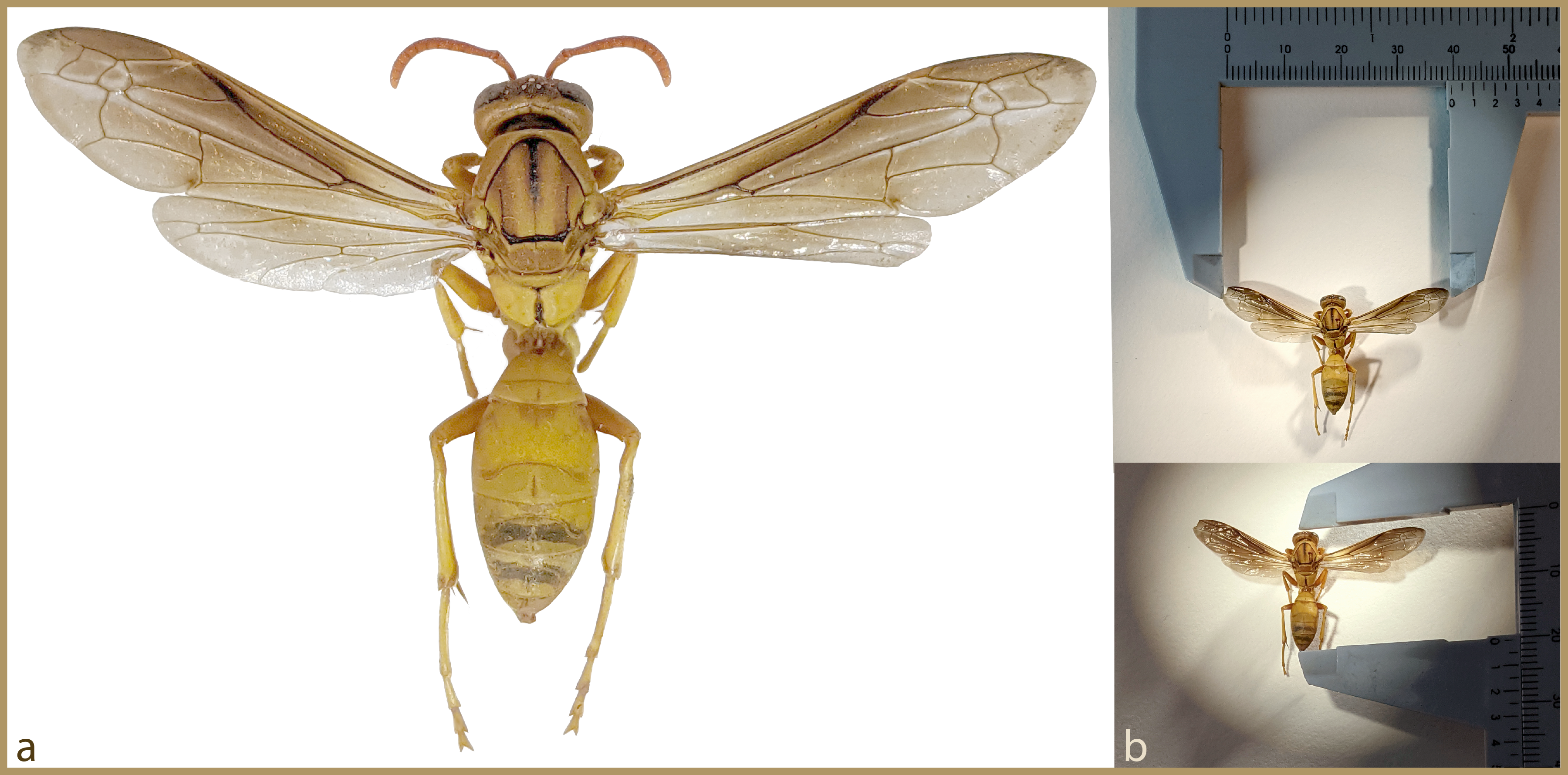
Figure 1. Polistes flavus paper wasp (Hymenoptera: Vespidae). Depending on how your specimen was preserved (frozen, in ethanol, dried and pinned), you can position it for optimal viewing and measuring. This can include positioning body and legs under alcohol so they are visible and bilaterally symmetrical, or (a) spread-mounting your specimen, as I did here after the wasp died and was frozen. (b) Calipers can be used to measure maximum width of specimen (top), and length of body (bottom). Next step: scale up these measurements for the illustration (Figure 2).
Note: I digitally “repaired” this damaged specimen for the purposes of this figure (e.g., by copying and pasting an antenna from another specimen), although damage and asymmetries still exist (e.g., right hindwing is damaged and pretarsi are missing).
(a) Measure the length of your insect. Calipers work well for making small measurements (Figure 1b), but carefully placing a little ruler immediately above or below the insect can also work. (If the insect is submerged in a transparent dish of liquid, the ruler can be seen below the specimen when placed below the dish.)
(b) Use a pencil and ruler to draw a vertical line down the center of your paper.
(c) Take the measurement you made of the insect and multiply that measurement by a whole number so the resulting measurement (and eventual drawing) will be large enough to fit nicely on your paper. Start by placing two dots on the vertical line to indicate the insect’s length (e.g., anterior end of head and posterior end of abdomen). For this specimen, I will scale up measurements by 7x.
(d) Measure lengths of each major segment along the body axis (e.g., length of head, middle section, and hind section of insect) and mark these, scaled up (7x, in our example), along the center line (Figure 2a).
(e) Now pick a few widths of your subject (e.g., widest part of head, widest part of prothorax, point of wing attachment, etc.), and place pairs of dots, equally spaced on either side of the vertical line to represent these widths (scaled up 3.5x to the left and 3.5x to the right of the vertical line, so the sum is 7x the width of whatever you chose to measure on the insect, to stick with the same 7x scaling example; Figure 2b). Each pair of dots should line up with a dot on the vertical line, measured to indicate where along the body axis the features of interest exist (e.g., where the head is widest). The more vertical and horizontal pairs of dots you create, the more your subject will become apparent. A million dots, and you’re done!
(f) Before you get carried away with your careful measurements, draw a light, rough pencil sketch of the outline of your subject to see how it will fit on your paper, leaving space on the edges of the paper (Figure 2c). A soft pencil (e.g., 2B) works best for this, and your hand should move across your paper with just enough force to create a line without embossing the paper.
(g) Start connecting the dots in light, sweeping motions. The left side will generally look like the mirror image of the right side (Figure 2d), so check to make sure what you’ve drawn on one side looks similar to the complementary features on the other side. One way to do this by eye is to cover one feature with your hand, look at the complementary feature as drawn on the other side, then lift your hand and look back at it. If this doesn’t help, you can photocopy, or photograph one side of your drawing, then horizontally flip the image and see how well it resembles the opposite side. If it is noticeably off, check your measurements. Does the head look too big relative to the thorax? Check your measurements.
The leap between steps c and d in Figure 2 might seem ludicrously large. What I omitted is merely the many incremental steps involving the same process of measuring and matching lengths and widths of left and right side until all desired components are positioned symmetrically and accurately.
Important note: Some features will not be symmetrical (e.g., the hemelytra of heteropteran true bugs), so don’t make the mistake of simply copying a tracing of one horizontally-flipped side.
5. Only when you are confident with your pencil drawing are you ready to replace pencil with ink or other media (e.g., color pencils, paint, etc.). I recommend starting with a simple, ink line drawing. Ink drawings are not as forgiving as some other media, but can be clean, clear, and easily reproduced. Using smooth strokes, go over your final pencil lines with a pen. I use Zig pens by Millennium (size 005) because they are acid-free, waterproof and alcohol-proof, and don’t smudge. Once finished, erase all pencil marks. Another option is to trace your pencil drawing with ink on tracing paper.
6. Scan your drawing, setting resolution to at least 300 ppi/dpi, and color to black and white (unless your drawing is in color). If the scan looks clean, and the image does not pixelate when zooming in a bit, you can import the scanned image into any number of programs (e.g., Gimp, Adobe Photoshop) to digitally clean the image (brightness, contrast, etc.) so that all that shows is the black and white of your ink on paper. Now is a good time to fix any errors made in ink by either using a digital erase tool or a paint tool. Resize and crop, as desired.
7. Include a labeled scale bar for size reference (scale bar instructions, below; Figure 3).
8. Create a figure legend (see examples, throughout).
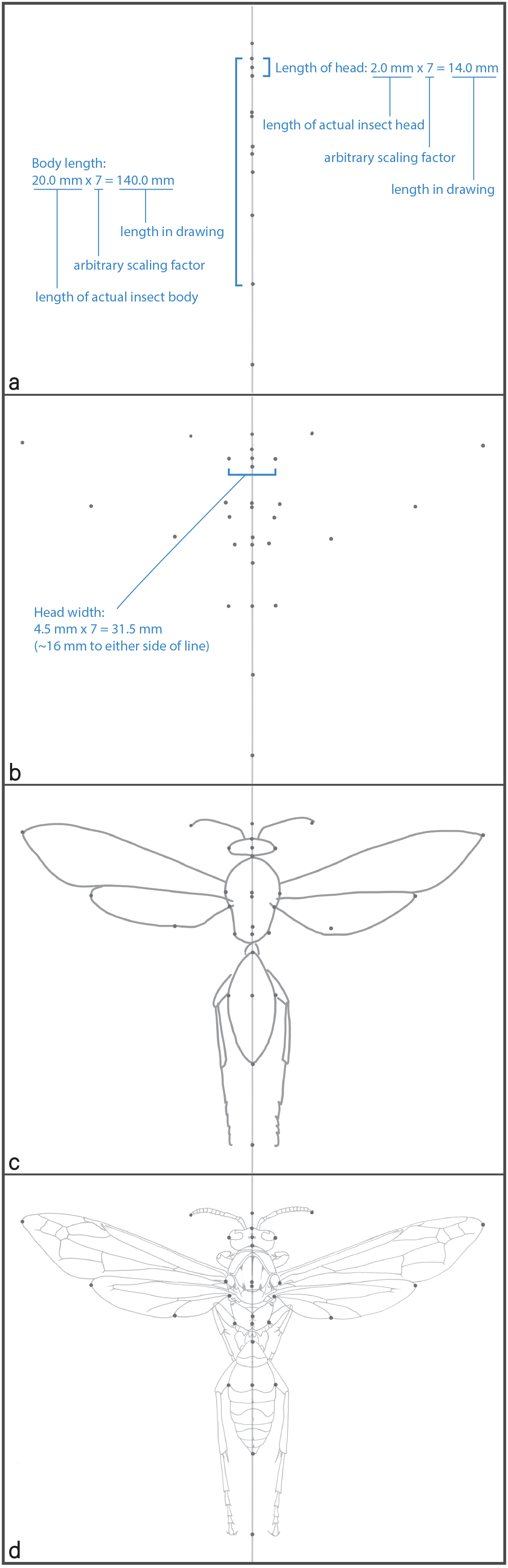
Figure 2. Steps that can be used to produce a proportionally-accurate scientific illustration, in this case of a paper wasp. Normally these images would be generated during the creation of the final illustration, but I created this figure using digital tools (Adobe Photoshop and Illustrator) for this newsletter article, long after having created the original illustration. See descriptions of (a) through (d) in text.
SCALE BAR INSTRUCTIONS When you look at an illustration of an organism, how can you tell how large the actual insect is? If the drawing of the insect is going to be 10 cm long (because that fits nicely on the paper, and will show enough detail), then the scale bar can tell a viewer how large the actual insect is that you drew. If the illustration is reproduced at a different size (like on a billboard), a viewer will always have this reference of scale.
First, decide how large you would like your drawing to be on your paper. It’s easiest to scale everything up by a whole number (e.g., 7x bigger than the original, as in our example above and below). The scale bar should be smaller than your drawn subject and a number that will be easy for a viewer to interpret and use; it should also be in metric units (e.g., mm or cm). Below is an example to illustrate this: The real paper wasp was originally only 2.0 cm long. I scaled up the wasp 7x in the drawing, so every part of the wasp should also be 7x longer than in the real wasp. Likewise, the scale bar that represents 1 cm must also be scaled by the same amount. In other words, a scale bar for 1 cm must be 7 cm.
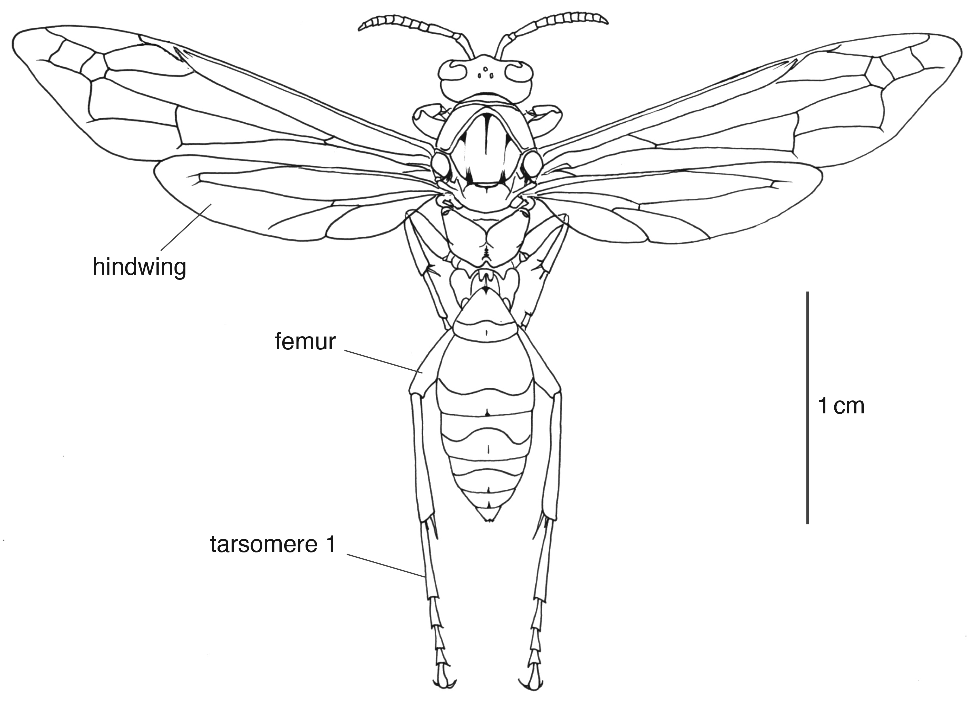
Figure 3. Dorsal view of female paper wasp, Polistes flavus (Order Hymenoptera, Family Vespidae). Illustration by Barrett Klein, 1999.
[This image is an example of a line drawing. Line drawings can be more or less detailed than this one.]
Modified from: Klein BA. 2003. Signatures of Sleep in the Paper Wasp Polistes flavus. Master’s thesis, University of Arizona, Tucson, AZ.
Another way you can think about scale bars is to use this equation:
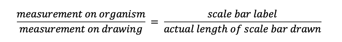
The length of the real wasp’s body is 2.0 cm, and the length of the wasp’s body in the drawing is 7x greater, or 14.0 cm. If we want a scale bar that we would label as 1 cm long (as in the drawing), we can figure out how long to draw that bar by setting up this equation:
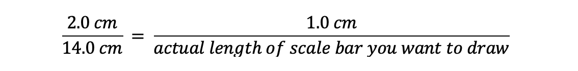
Solve for x and you find that x = 7, so you should draw your scale bar 7 cm long if you want to label it 1 cm.
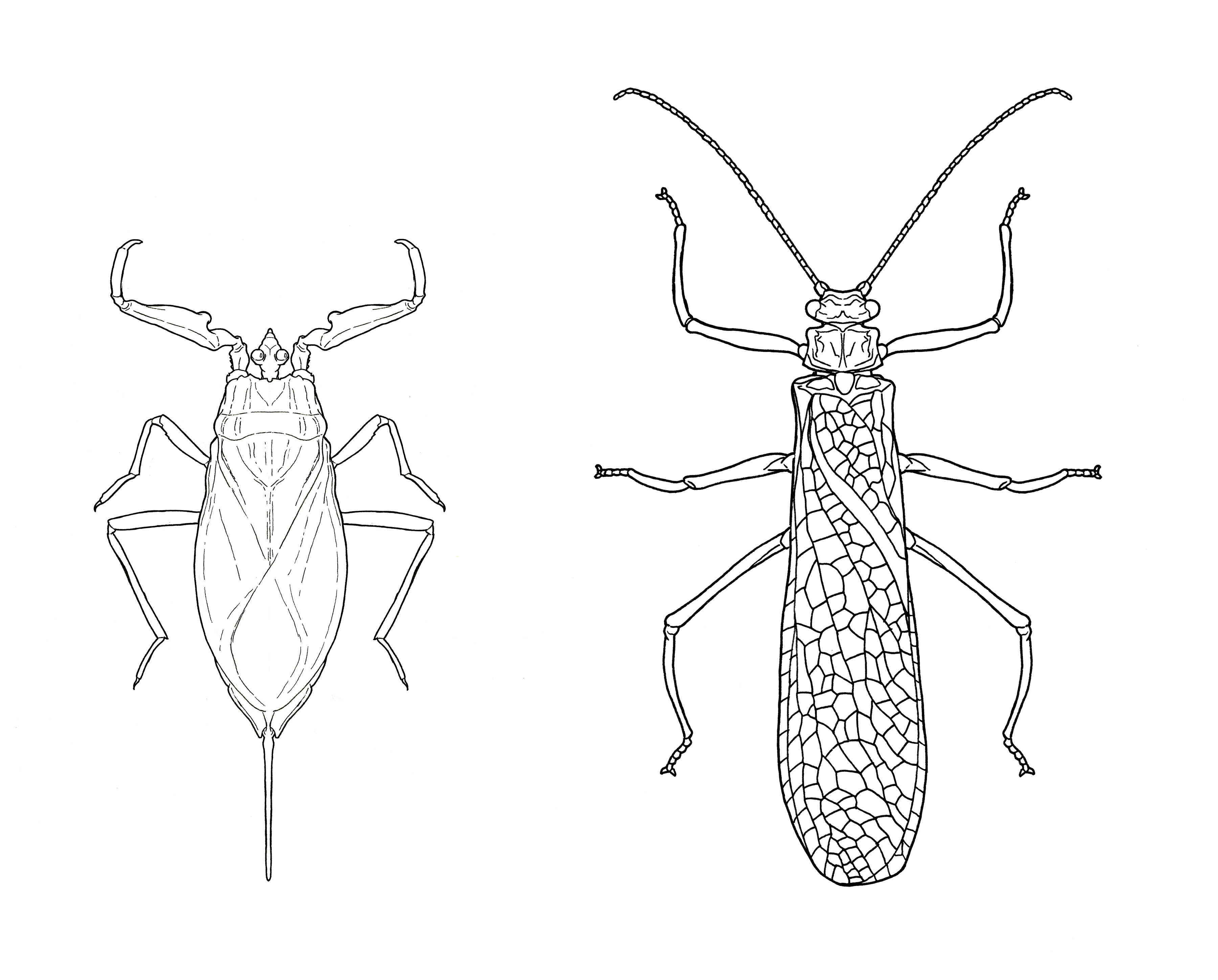
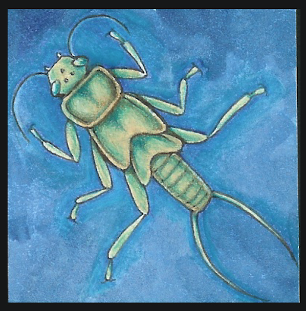
Figure 4. Dorsal view of two aquatic (finally!) insects. Illustrations by Matthew Sigrist, 2020.
[These are two more examples of line drawings. Matthew Sigrist produced these using similar techniques as outlined here, but digitally flipped half of each drawing to achieve symmetry, where symmetry is supposed to exist. “With many of these illustrations of a dorsal view, I focus on fully rendering only one half of the sketch to be digitally mirrored over the animal's line of symmetry later; in the case of these nepid and stonefly illustrations, I varied from this method slightly by drawing the full asymmetrical wings and later mirroring only those other features which are reflected over the insect's line of symmetry.”]
Line drawings are especially useful for clearly showing salient features of your subject, but sometimes other methods are necessary for communicating key features. Below are three alternative approaches to depicting adult insects – with color, with more three-dimensional detail/texture, or produced entirely digitally.
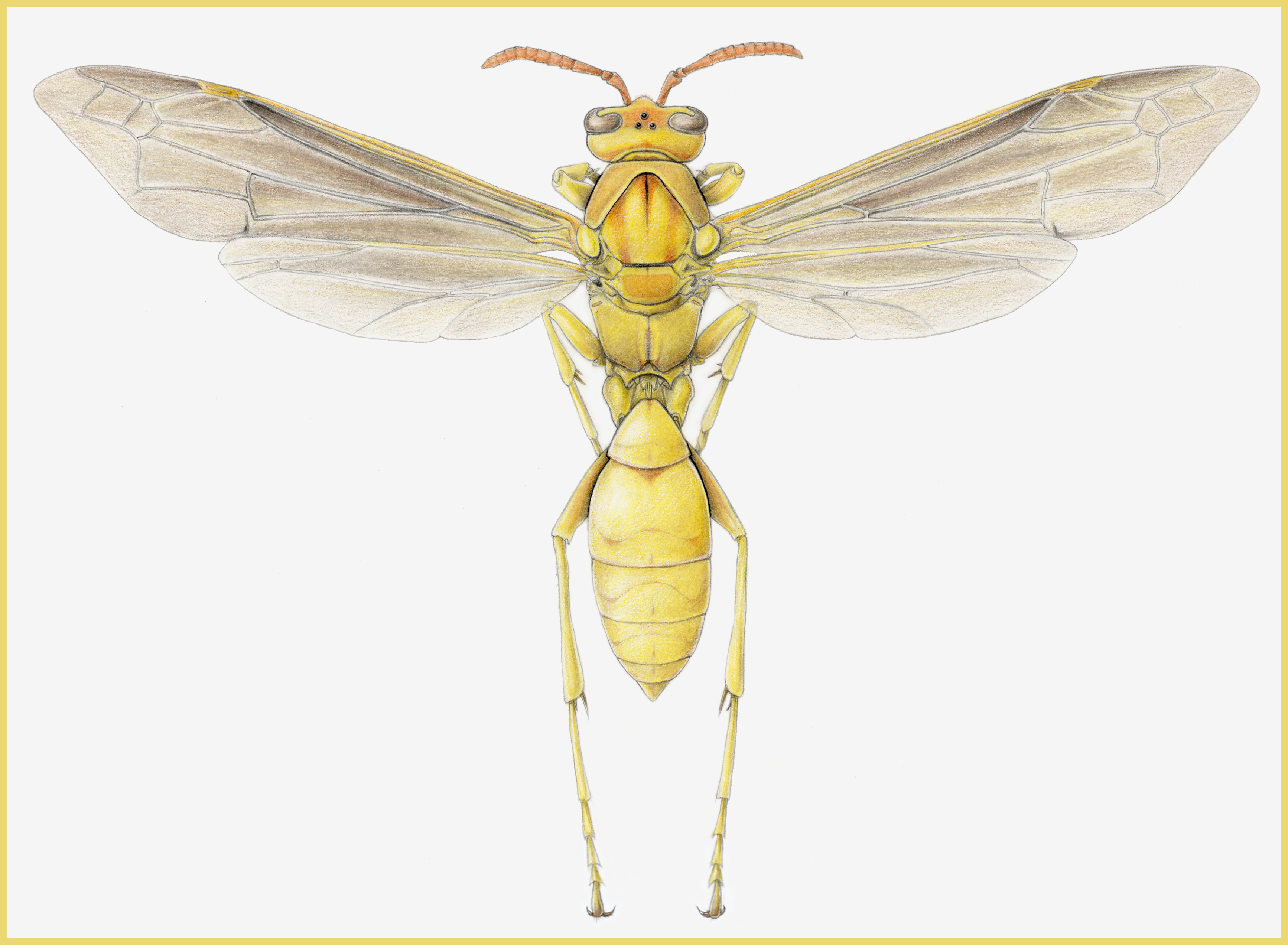
Figure 5. Here is the same wasp as depicted in Figure 3, but now in color, using color pencils instead of pen and ink. The wasp is named Polistes flavus, and “flavus” refers to its yellow coloration, an identifying characteristic absent in the pen and ink version. Illustration by Barrett Klein, 1999.
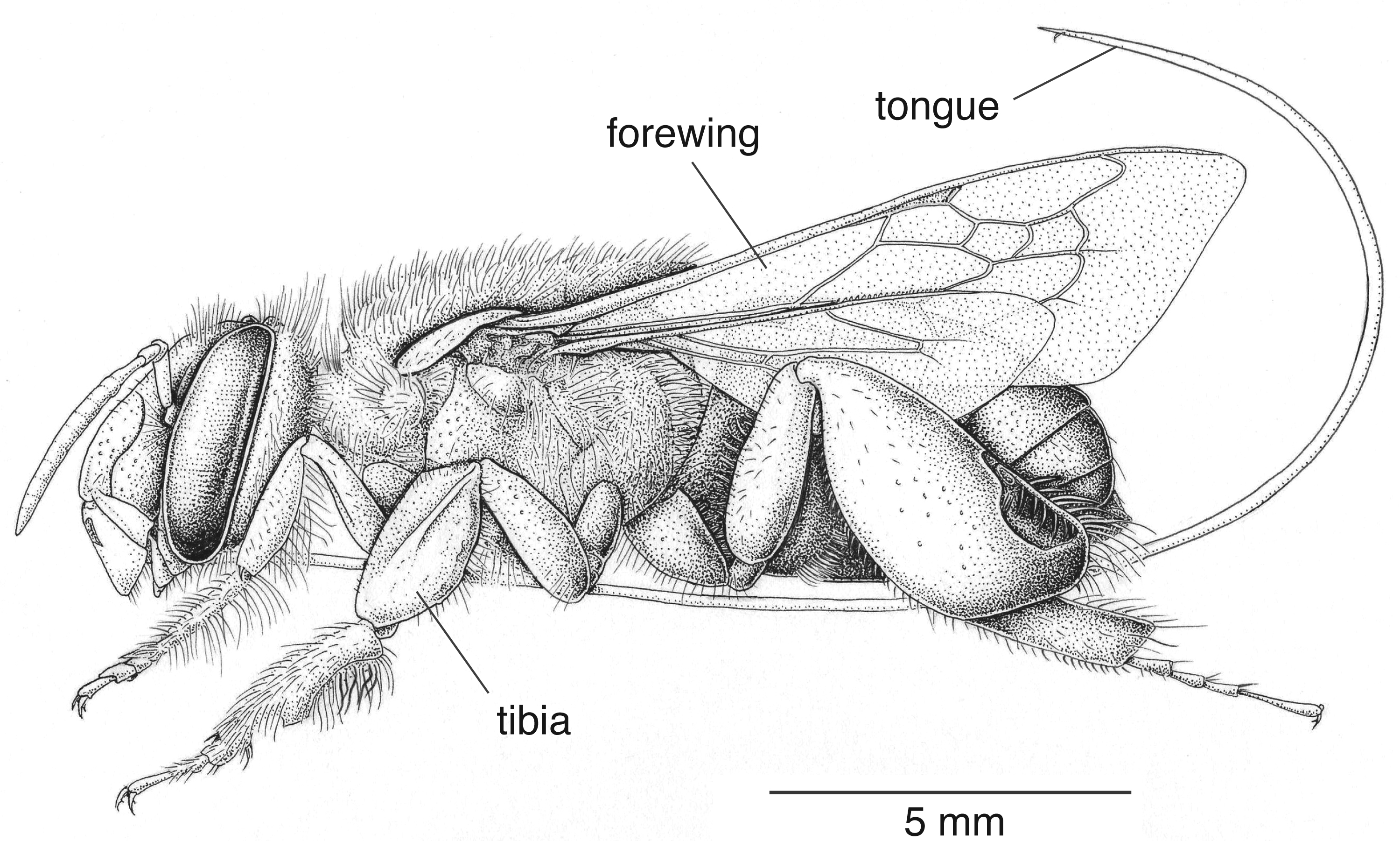
Figure 6. Lateral view of male Euglossa hugonis orchid bee. Illustration by Barrett Klein, 2003.
[This image is an example of a more detailed, stippled drawing in which the (lateral) view does not allow for symmetrical measurements, as outlined above.]
Modified from source: Roubik DW. 2004. Sibling species among Glossura and Glossuropoda in the Amazon region (Hymenoptera; Apidae: Euglossini). Journal of the Kansas Entomological Society. 77:235-253.
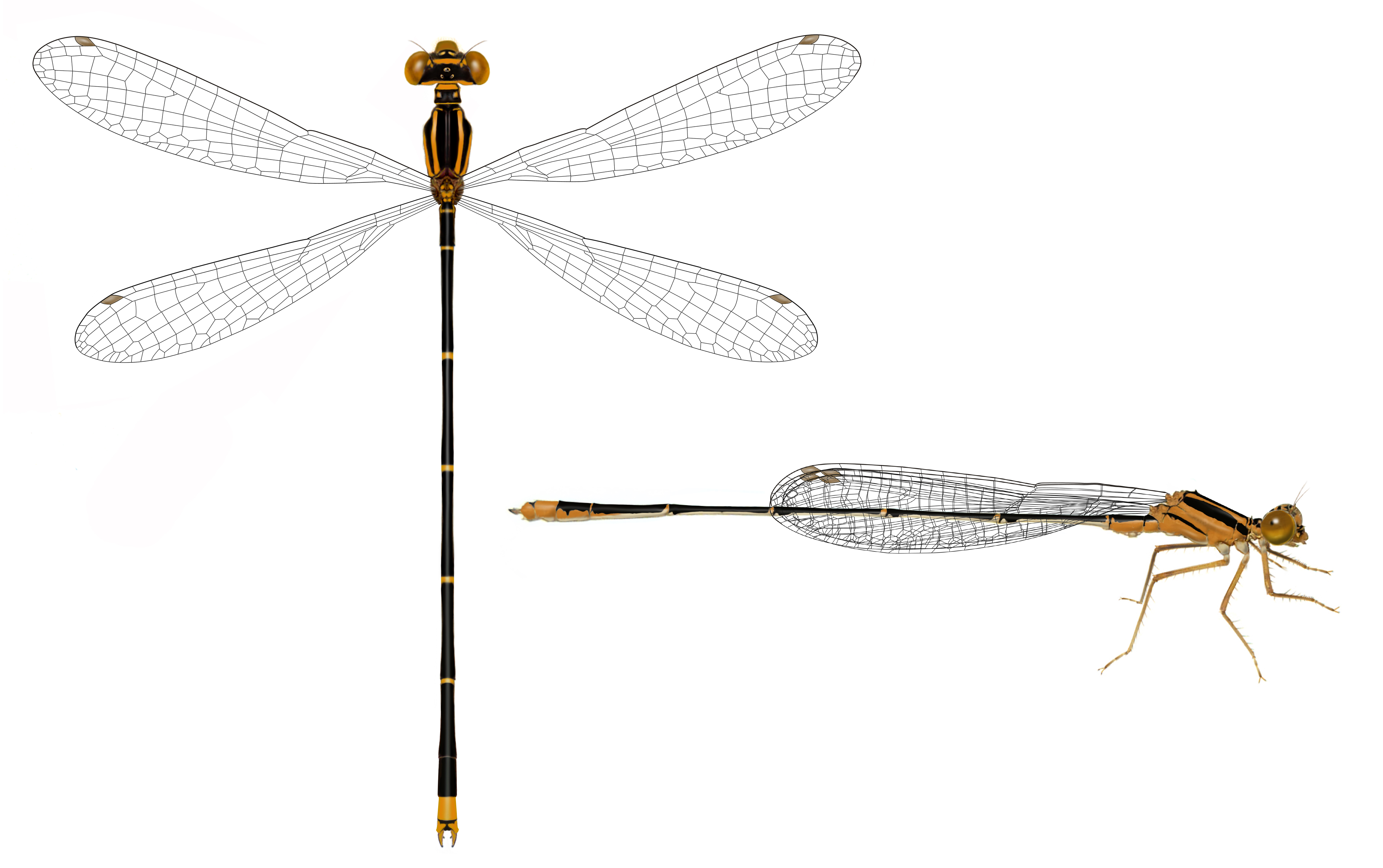
Figure 7. Dorsal and lateral view of Enallagma truncatum, a damselfly endemic to western Cuba and thought to be extinct. Illustrations by Barrett Klein, 2021.
[These images were created an entirely different way, by starting with photographs of a dried and dingy dead specimen and digitally resurrecting the specimen by assembling, cleaning, and painting in Adobe Photoshop.]
Source: To be published in Libélulas de Cuba, with permission from the author, Adrian Trapero-Quintana.
VOILÀ! YOU’RE A SCIENTIFIC ILLUSTRATOR!
If this lesson merely frustrated you, do not despair! Don’t shy away from practicing and presenting your growing skills as a visual communicator of science. Please explore professional organizations’ online resources (see references) and published guides (e.g., Hodges 2003), and practice using whatever media excites you. Some professional scientific illustrators rarely touch a pencil, preferring to work entirely digitally. Others combine traditional and modern techniques and approaches. Remember, the primary message of this post is for you to advance your science by conveying your message visually. Whether you are using age-old or cutting-edge tools, with practice you will be able to visually entice and educate your audience.
Acknowledgments: Angele Mele, Korinthia Klein, Arno Klein, Danielle VanBrabant, Damond Kyllo, and Dosha Klein offered valuable suggestions to an earlier draft of this post, convincing me that I will need to create an expanded version of this in the future. Pupating Eufinger and Matthew Sigrist graciously supplied images. Thank you to Adrian Trapero-Quintana for allowing me to include images of the Cuban damselfly prior to the publication of his book. Some elements of this introduction to scientific illustration come from an Organismal Biology lab exercise I wrote with Meredith Thomsen and other wonderful colleagues at the University of Wisconsin – La Crosse.
References
Hodges, E.A. 2003. The Guild Handbook of Scientific Illustration, 2nd ed. Wiley & Sons, Inc. NJ, USA.
Wong, B. 2011. Layout. Nature Methods. 8:783. (and all of Bang Wong’s one-page lessons in Nature Methods)
Associations
Guild of Natural Science Illustrators https://www.gnsi.org/ American Society of Botanical Artists https://www.asba-art.org/ Association of Medical Illustrators https://www.ami.org/
Additional online resources
GNSI listserv https://www.gnsi.org/listserv Art & Science Collaborations, Inc. (ASCI) http://www.asci.org/ Sciart Magazine https://www.sciartmagazine.com/
SFS Request for Proposals
The Long-Range Planning Committee (LRPC) is requesting proposals from SFS members for projects that make progress towards achieving the Society’s strategic goals, as detailed in the 2020-2025 SFS Strategic Plan. Proposals will be due by August 20, 2021. Please email proposals as a single PDF file to Todd Royer, LRPC co-chair, troyer@indiana.edu.
Article Spotlight
By Ali Chalberg
![]()
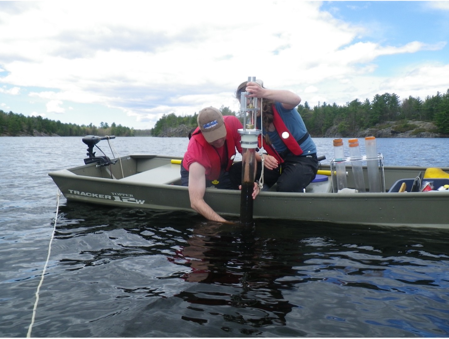
Road salts are commonly used in northern climates winter road maintenance. Salts can be washed off of the roads and into our aquatic systems, especially in urban areas. Increasing the salinity of aquatic systemsand can negatively affect the organisms that live in these areas. In this study, the authors looked at the long-term effects that road salts have on zooplankton in Ontario, Canada.
Lead author, Robin Valleau, is a PhD. candidate at Queen’s University in Ontario Canada. Robin’s co-author and advisor, Dr. John P. Smol, is a distinguished university professor as well as the Canada research chair in environmental change at Queen’s University. Along with co-author Andrew Paterson, their research focuses on using paleolimnology to understand how road salt has impacted cladocerans in shallow Precambrian Shield lakes.
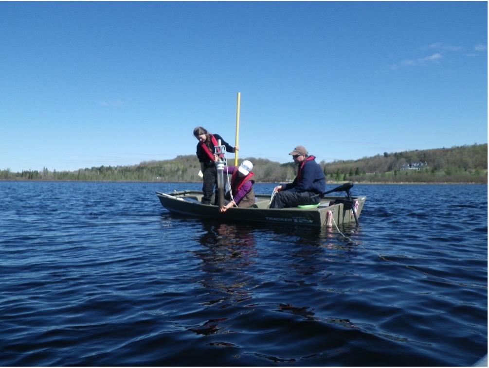
Field work sampling on Jevins Lake, Pictured is Robin Valleau, Anna DeSellas, and Andrew Paterson
Picture Credit: Mark Gilies
Paleolimnological studies use lake sediment layers to understand the history of lakes. Dr. Smol likens this to that of forensic work, as you have an event that occurred, and you have to go look back in time to see what the cause was. In this case with a sediment core, they are able to section it by time and within those sections, categorize the zooplankton. From this you are able to see changes in a population over time with increasing levels of chloride.
Their study is unique as it is one of the first studies to look at the effect’s chloride concentrations have had on zooplankton over a long-term time scale. They hypothesized that softwater lakes would see a greater impact with an increase in chloride. They found that zooplankton were reacting to chloride well below the water quality guidelines which means zooplankton assemblages were negatively affected.
Studies such as these illustrate the need for region specific guidelines in regard to environmental regulations. As Dr. Smol stated, “Not every lake is the same” so they need to be managed differently. Robin emphasized the need to use regionally specific species when setting water quality guidelines as most guidelines focus on daphnia that are not readily found in many of these lakes. Ecological studies such as this are important as they paint a picture of “where we have come from and where we are going” which is at the heart of management.
Sampling of sediment cores on Jevins Lake in Ontario Canada. Picture credit: Mark Gilies
This study has inspired other research. For example, they observed bosmina were heavily impacted by chloride, so they are currently performing laboratory studies to measure zooplankton's tolerance to road salt.
To conclude I asked Dr. Smol for some advice for up-and-coming scientists. He eagerly “Do what you're interested in and what you love because if you're interested in it, you'll probably be good at it!” Finally, he would like everyone to remember “if you get a lucky break, run with it!”
You can read the journal article in Freshwater Science at: https://www.journals.uchicago.edu/doi/10.1086/711666
Children's Book
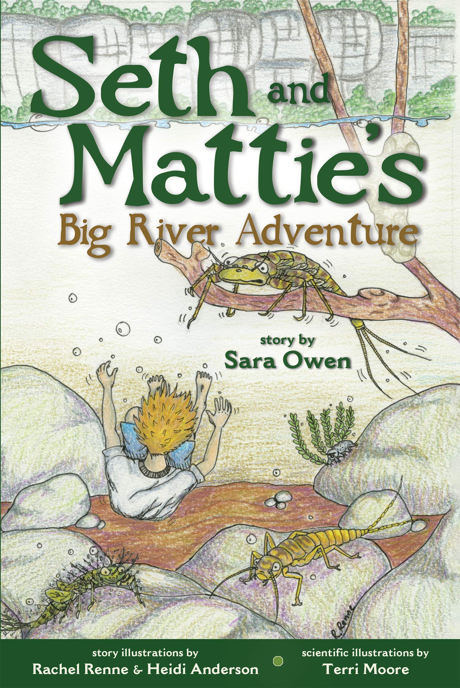
Seth and Mattie's Big River Adventure is a giant, underwater escapade that offers readers 8-12 a close-up view of the river's smallest inhabitants, and even includes an illustrated glossary featuring the book's Cast of Characters. Throughout his thrilling and educational tour of the river's ecosystem, Seth encounters the unknown and unexpected with a courage, enthusiasm, and wonder that will inspire other young explorers en route to their next great discovery!
Documentary Go Fund Me

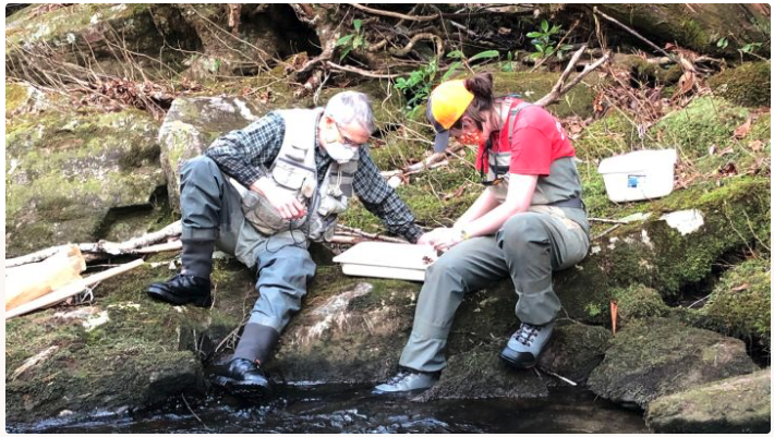
Help fund a documentary: For 30 years, Dr. John Morse has taught Aquatic Entomology at Highlands Field Station in North Carolina. This summer will be year 31. If you took Dr. Morse's EPT course you remember how tough it was: 12-14 hours a day, every day, for two weeks! We want to make a short documentary to tell John's story and capture the adventure of the most popular course the field station has ever seen.
Every donation counts!!
Book Review
By Amy Rosemond
Professor, Odum School of Ecology, University of Georgia, Athens, GA USA 30622
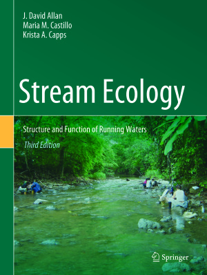
New textbook to understand & conserve stream ecosystems!
Reading the reviews from J. David Allan’s 1st edition of Stream Ecology (1995) feels downright quaint. At that time, the field of stream ecology had emerged as a discipline from its roots in hydrology, geomorphology, biogeochemistry and bioassessment, coupled with the natural history observations of amateur fly fishers and professional zoologists. Allan’s book was seen as the successor to Hynes’ 1971 text, The Ecology of Running Waters. The science was fledging and Allan’s book did a lot to help launch us all from the nest by describing a quantitative and interdisciplinary approach to understanding streams. It guided us as we pondered the strengths of biotic vs abiotic control, when and where the River Continuum Concept applied to streams, described functional feeding groups of macroinvertebrates, and more. Those steps, along with advances in technologies, modeling, and frameworks that many in our Society have developed in subsequent decades, have given us new tools to understand streams. In the 3rd edition of Stream Ecology, Allan, with co-authors Maria M. Castillo and Krista A Capps, successfully captures not only the scale of these advances, but also the scale of the challenges we still need to address.
The authors have compiled a hefty yet accessible volume, organized into 15 chapters. It opens with the context of Rivers in the Anthropocene, followed by physical-chemical aspects (streamflow, geomorphology, sediment, chemistry, other abiotic characterization), biological structural components (primary producers, detritus, microbial ecology), community and food web interactions (trophic relationships, species interactions, communities) and ecosystem processes (energy flow, nutrient cycling, carbon and stream metabolism). The final chapter is How We Manage Rivers and Why. The organization is logical and the treatment is comprehensive. The authors should be commended for the rich examples from the recent literature, including figures and tables that introduce concepts such as ELOHA (ecological limits of hydrologic alteration) and the freshwater salinization syndrome. Chapters include well-illustrated and up-to-date treatment of topics ranging from emerging contaminants to controls on species and community assembly, and methodologies for measuring nutrient uptake and metabolism.
The difference between the 1st and 3rd editions of Stream Ecology illustrates not only how profoundly the world has changed in the past 25+ years, but also how our science has been motivated and inspired by those challenges. Scientifically, we have not been asleep at the wheel. As individuals, we also recognize the limits to science that have resulted in inadequate and unjust solutions to growing freshwater challenges. The book makes excellent progress on citing new voices and scientific advances. As likely envisioned by the authors, new generations of scientists will ideally use this volume as a guidebook and foundation to broaden the scope and effectiveness of our field.
The book is available in hardback for $139 USD (ISBN 978-3-030-61285-6) and as an ebook for $109 (978-3-030-61286-3). Individual chapters are available to purchase separately. This book is also available for sale at the virtual meeting.
2021 Annual Meeting Recap
Great Faces
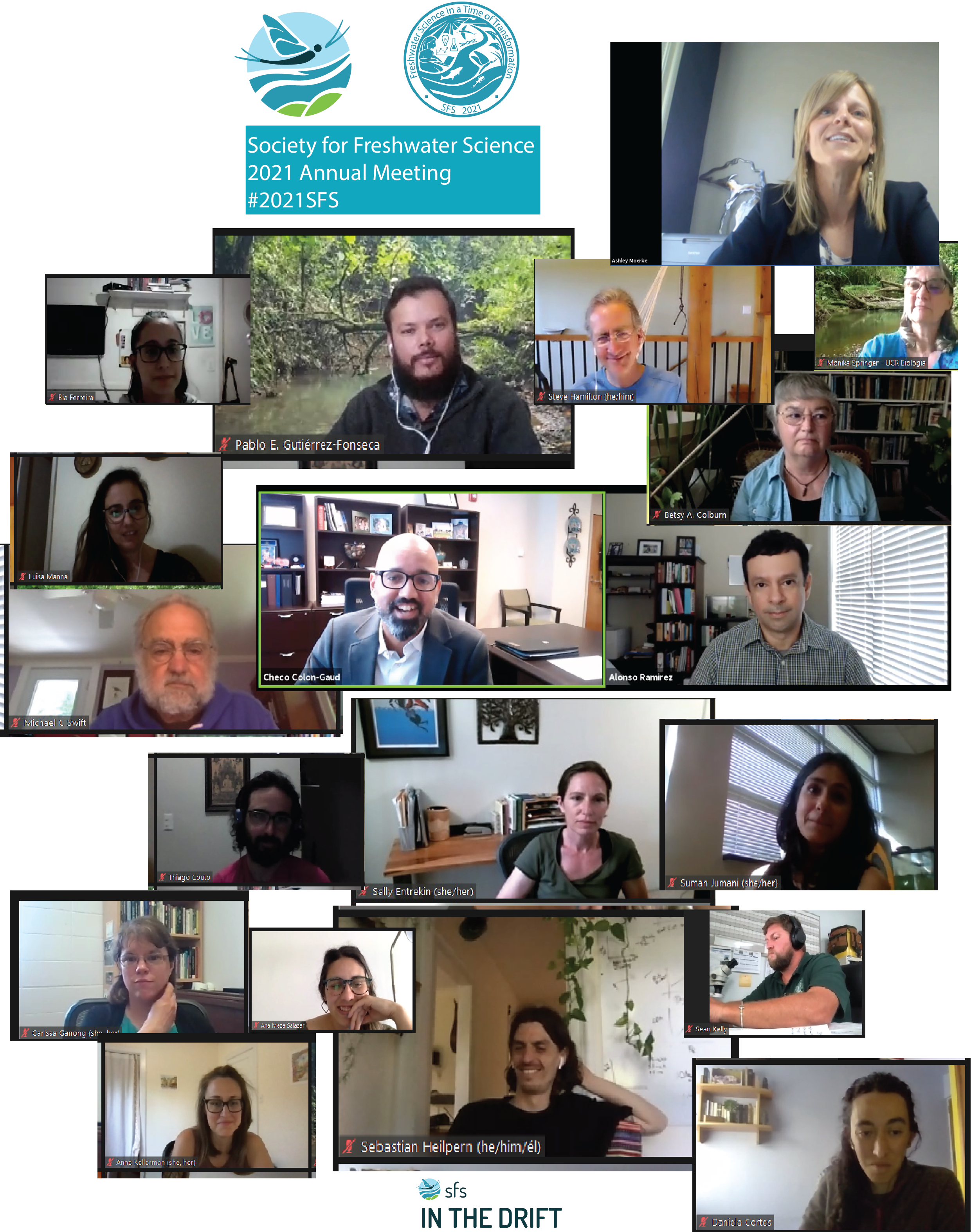
Inspiring Plenaries

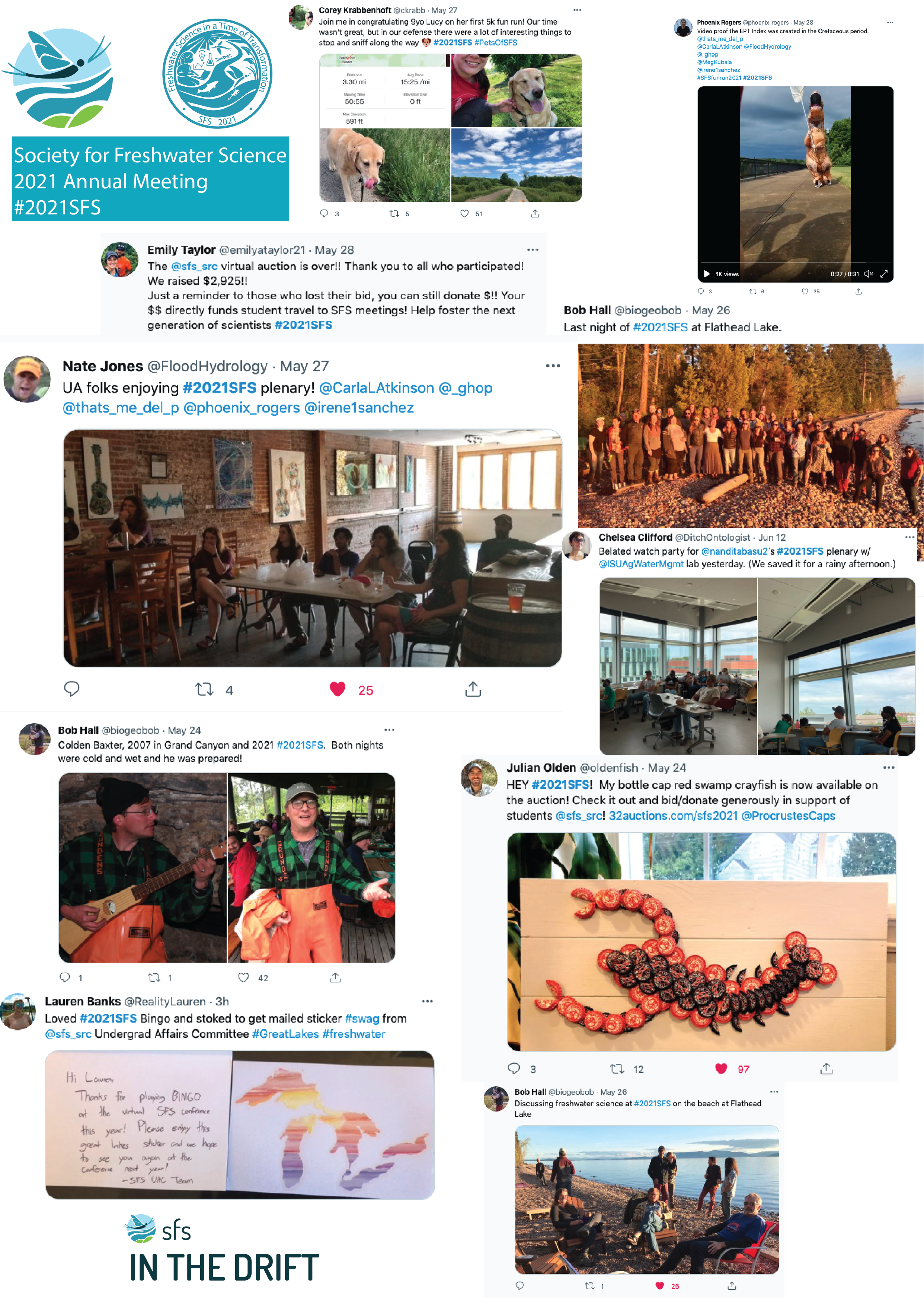
Watch Parties and Social Media
Awards and Acknowledgments